[1]:

#@title
#
# Licensed under the Apache License, Version 2.0 (the "License");
# you may not use this file except in compliance with the License.
# You may obtain a copy of the License at
#
#     http://www.apache.org/licenses/LICENSE-2.0
#
# Unless required by applicable law or agreed to in writing, software
# distributed under the License is distributed on an "AS IS" BASIS,
# WITHOUT WARRANTIES OR CONDITIONS OF ANY KIND, either express or implied.
# See the License for the specific language governing permissions and
# limitations under the License.

k-means clustering

Download the tutorial as a Jupyter notebook

In this tutorial, we will use the NeoML implementation of k-means clustering algorithm to clusterize a randomly generated dataset.

The tutorial includes the following steps:

Generate the dataset
Cluster the data
Visualize the results

Generate the dataset

Note: This section doesn’t have any NeoML-specific code. It just generates a dataset. If you are not running this notebook, you may skip this section.

Let’s generate a dataset of 4 clusters on the plane. Each cluster will be generated from center + noise taken from normal distribution for each coordinate.

[2]:

import numpy as np

np.random.seed(451)

n_dots = 128
n_clusters = 4
centers = np.array([(-2., -2.),
                   (-2., 2.),
                   (2., -2.),
                   (2., 2.)])
X = np.zeros(shape=(n_dots, 2), dtype=np.float32)
y = np.zeros(shape=(n_dots,), dtype=np.int32)

for i in range(n_dots):
    # Choose random center
    cluster_id = np.random.randint(0, n_clusters)
    y[i] = cluster_id
    # object = center + some noise
    X[i, 0] = centers[cluster_id][0] + np.random.normal(0, 1)
    X[i, 1] = centers[cluster_id][1] + np.random.normal(0, 1)

Cluster the data

Now we’ll create a neoml.Clustering.KMeans class that represents the clustering algorithm, and feed the data into it.

[3]:

import neoml

kmeans = neoml.Clustering.KMeans(max_iteration_count=1000,
                                 cluster_count=n_clusters,
                                 thread_count=4)
y_pred, centers_pred, vars_pred = kmeans.clusterize(X)

Before going further let’s take a look at the returned data.

[4]:

print('y_pred')
print('  ', type(y_pred))
print('  ', y_pred.shape)
print('  ', y_pred.dtype)

print('centers_pred')
print('  ', type(centers_pred))
print('  ', centers_pred.shape)
print('  ', centers_pred.dtype)

print('vars_pred')
print('  ', type(vars_pred))
print('  ', vars_pred.shape)
print('  ', vars_pred.dtype)

y_pred
   <class 'numpy.ndarray'>
   (128,)
   int32
centers_pred
   <class 'numpy.ndarray'>
   (4, 2)
   float64
vars_pred
   <class 'numpy.ndarray'>
   (4, 2)
   float64

As you can see, the y_pred array contains the cluster indices of each object. centers_pred and disps_pred contain centers and variances of each cluster.

Visualize the results

In this section we’ll draw both clusterizations: ground truth and predicted.

[5]:

%matplotlib inline

import matplotlib.pyplot as plt

colors = {
    0: 'r',
    1: 'g',
    2: 'b',
    3: 'y'
}

# Create figure with 2 subplots
fig, axs = plt.subplots(ncols=2)
fig.set_size_inches(10, 5)

# Show ground truth
axs[0].set_title('Ground truth')
axs[0].scatter(X[:, 0], X[:, 1], marker='o', c=list(map(colors.get, y)))
axs[0].scatter(centers[:, 0], centers[:, 1], marker='x', c='black')

# Show NeoML markup
axs[1].set_title('NeoML K-Means')
axs[1].scatter(X[:, 0], X[:, 1], marker='o', c=list(map(colors.get, y_pred)))
axs[1].scatter(centers_pred[:, 0], centers_pred[:, 1], marker='x', c='black')

plt.show()

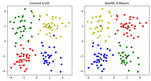
As you can see, k-means didn’t clusterize the outliers correctly.